We have already covered the majority of the exercises in week 4. This week, we will focus on an advanced performance concept that is not covered anywhere else in the course: branch prediction.
Take a look at the following Rcpp code:
#include <Rcpp.h>// Count > threshold with a hard branchint count_branchy(Rcpp::NumericVector x,double t){int n = x.size(), cnt =0;for(int i =0; i < n;++i){if(x[i]> t)++cnt;}return cnt;}// Count > threshold without a hard branchint count_branchless(Rcpp::NumericVector x,double t){int n = x.size(), cnt =0;for(int i =0; i < n;++i){ cnt +=(x[i]> t);}return cnt;}// Two-path summation (branchy)double sum_branchy(Rcpp::NumericVector x,double thr){double s =0.0;for(int i =0; i < x.size();++i){double xi = x[i];if(xi >= thr) s += xi;else s +=2.0* xi;}return s;}// Two-path summation (branchless)double sum_branchless(Rcpp::NumericVector x,double thr){double s =0.0;for(int i =0; i < x.size();++i){double xi = x[i];double mask =(xi >= thr); s += mask * xi +(1.0- mask)*(2.0* xi);}return s;}
In the code above, we have two functions that count the number of elements in a vector that are greater than a threshold, and two functions that sum the elements in a vector that are greater than a threshold. The functions come in two flavors: one that uses an if statement, and another that uses a mask.
In the if statement version, code is executed conditionally based on the result of a comparison. In the mask version, one applies a mask to the elements of the vector, and then adds the mask to the sum.
What exactly is branch prediction?
When a computer runs code with an if statement (a “branch”), it has to decide what to do next: take one path, or the other. Modern computer processors (CPUs) are designed to run instructions very quickly and efficiently. But when they reach a branch (like an if statement), they attempt to guess which direction the code will take. This is called branch prediction.
If the CPU’s guess is correct, everything runs smoothly and quickly. However, if the guess is wrong, the processor has to throw away some of the work it started and do it over. This can slow down your code, especially if there are many unpredictable branches.
For statisticians, this matters because many statistical and data-wrangling tasks involve checking conditions repeatedly (like whether data points pass a threshold, or which group an observation belongs to). Understanding branch prediction helps us write code that the computer can run faster—especially for large datasets or simulations.
The code above illustrates two styles: one that uses explicit branches (if statements), and another that uses arithmetic “masks” to avoid branches. The version without branches can run faster on modern CPUs, especially when the branch direction is hard to predict.
set.seed(1)n <-5e6# Case A: "Always true" branch (maximally predictable)# Pick a very low threshold so every comparison is truex_any <-rnorm(n)thr_all_true <--1e9# Case B: Single flip (long runs -> easy prediction)# First 99.9% below thr, last 0.1% above thrthr_split <-0.0x_easy <-c(rep(-1.0, n -5000L), rep(1.0, 5000L))# Case C: Hard 50/50 random (for contrast)x_rand <-rnorm(n)thr_med <-0.0# Warm-upinvisible(count_branchy(x_any, thr_all_true))invisible(count_branchless(x_any, thr_all_true))invisible(sum_branchy(x_any, thr_all_true))invisible(sum_branchless(x_any, thr_all_true))# Benchmarks where BRANCHY SHOULD WIN or TIEbench_easy_counts <- bench::mark(branchy_all_true =count_branchy(x_any, thr_all_true),branchless_all_true =count_branchless(x_any, thr_all_true),branchy_singleflip =count_branchy(x_easy, thr_split),branchless_singleflip =count_branchless(x_easy, thr_split),iterations =30, check =FALSE, min_time =0.5)bench_easy_sums <- bench::mark(sum_branchy_all_true =sum_branchy(x_any, thr_all_true),sum_branchless_all_true =sum_branchless(x_any, thr_all_true),sum_branchy_singleflip =sum_branchy(x_easy, thr_split),sum_branchless_singleflip =sum_branchless(x_easy, thr_split),iterations =30, check =FALSE, min_time =0.5)# Contrast: hard 50/50 case where BRANCHLESS SHOULD WINbench_hard_counts <- bench::mark(branchy_random =count_branchy(x_rand, thr_med),branchless_random =count_branchless(x_rand, thr_med),iterations =30, check =FALSE, min_time =0.5)bench_hard_sums <- bench::mark(sum_branchy_random =sum_branchy(x_rand, thr_med),sum_branchless_random =sum_branchless(x_rand, thr_med),iterations =30, check =FALSE, min_time =0.5)bench_easy_counts
# A tibble: 4 × 6
  expression                 min   median `itr/sec` mem_alloc `gc/sec`
  <bch:expr>            <bch:tm> <bch:tm>     <dbl> <bch:byt>    <dbl>
1 branchy_all_true        3.71ms   3.76ms      264.        NA        0
2 branchless_all_true     3.72ms   3.96ms      255.        NA        0
3 branchy_singleflip       3.7ms   3.76ms      266.        NA        0
4 branchless_singleflip   3.74ms   3.76ms      263.        NA        0
bench_easy_sums
# A tibble: 4 × 6
  expression                     min   median `itr/sec` mem_alloc `gc/sec`
  <bch:expr>                <bch:tm> <bch:tm>     <dbl> <bch:byt>    <dbl>
1 sum_branchy_all_true        18.7ms   18.8ms      53.2        NA        0
2 sum_branchless_all_true     18.7ms   18.8ms      52.9        NA        0
3 sum_branchy_singleflip      18.7ms   18.8ms      53.3        NA        0
4 sum_branchless_singleflip   18.7ms   18.8ms      53.2        NA        0
bench_hard_counts
# A tibble: 2 × 6
  expression             min   median `itr/sec` mem_alloc `gc/sec`
  <bch:expr>        <bch:tm> <bch:tm>     <dbl> <bch:byt>    <dbl>
1 branchy_random       3.7ms   3.75ms      267.        NA        0
2 branchless_random   3.75ms   3.77ms      265.        NA        0
bench_hard_sums
# A tibble: 2 × 6
  expression                 min   median `itr/sec` mem_alloc `gc/sec`
  <bch:expr>            <bch:tm> <bch:tm>     <dbl> <bch:byt>    <dbl>
1 sum_branchy_random      38.4ms   38.4ms      26.0        NA        0
2 sum_branchless_random   40.7ms     41ms      24.4        NA        0
From the results, we see that the branchless version is faster than the branchy version in all cases. The prformance difference is double in the random cases, since the branch direction is completely unpredictable. Whereas in the easy cases, where one branch is taken >99% of the time, we see that the difference is quite small.
It is important to keep in mind that this is a very simple example, and in certain real world cases, the branchy version may be faster!
Rejection sampling and branch prediction
Now let’s apply the branch prediction concept to rejection sampling. In rejection sampling, we repeatedly generate proposals and accept or reject them based on some criterion. This naturally involves branching - either we accept the proposal or we reject it and try again.
Visualizing the Target Density and Proposal Distribution
To better understand how rejection sampling works, let’s first visualize the target density and the proposal distribution together. This helps us see how well the proposal distribution “envelopes” the target density.
# Load the datapoisson_data <-read.csv(here::here("data", "poisson.csv"))x <- poisson_data$xz <- poisson_data$z# Check that data loaded correctlycat("Data loaded successfully. x has", length(x), "values, z has", length(z), "values\n")
Data loaded successfully. x has 100 values, z has 100 values
# Define the target density function (unnormalized) - same as in presentationf_dens1 <-function(y, x, z) prod(exp(y * z * x -exp(y * x)))f_dens1 <-Vectorize(f_dens1, vectorize.args ="y")# Create sequence for optimization and plottingx_seq <-seq(0, 1, 0.001)# Find optimal mean: mu^opt = argmax f_dens1(x)mu_opt <- x_seq[which.max(f_dens1(x_seq, x, z))]cat("Optimal mean (mu_opt):", mu_opt, "\n")
# Sanity check: envelope should be larger than targetenvelope_check <-min(dnorm(x_seq, mu_opt, sd_opt) -f_dens1(x_seq, x, z) * alpha_opt)cat("Envelope check (should be >= 0):", envelope_check, "\n")
Envelope check (should be >= 0): 0
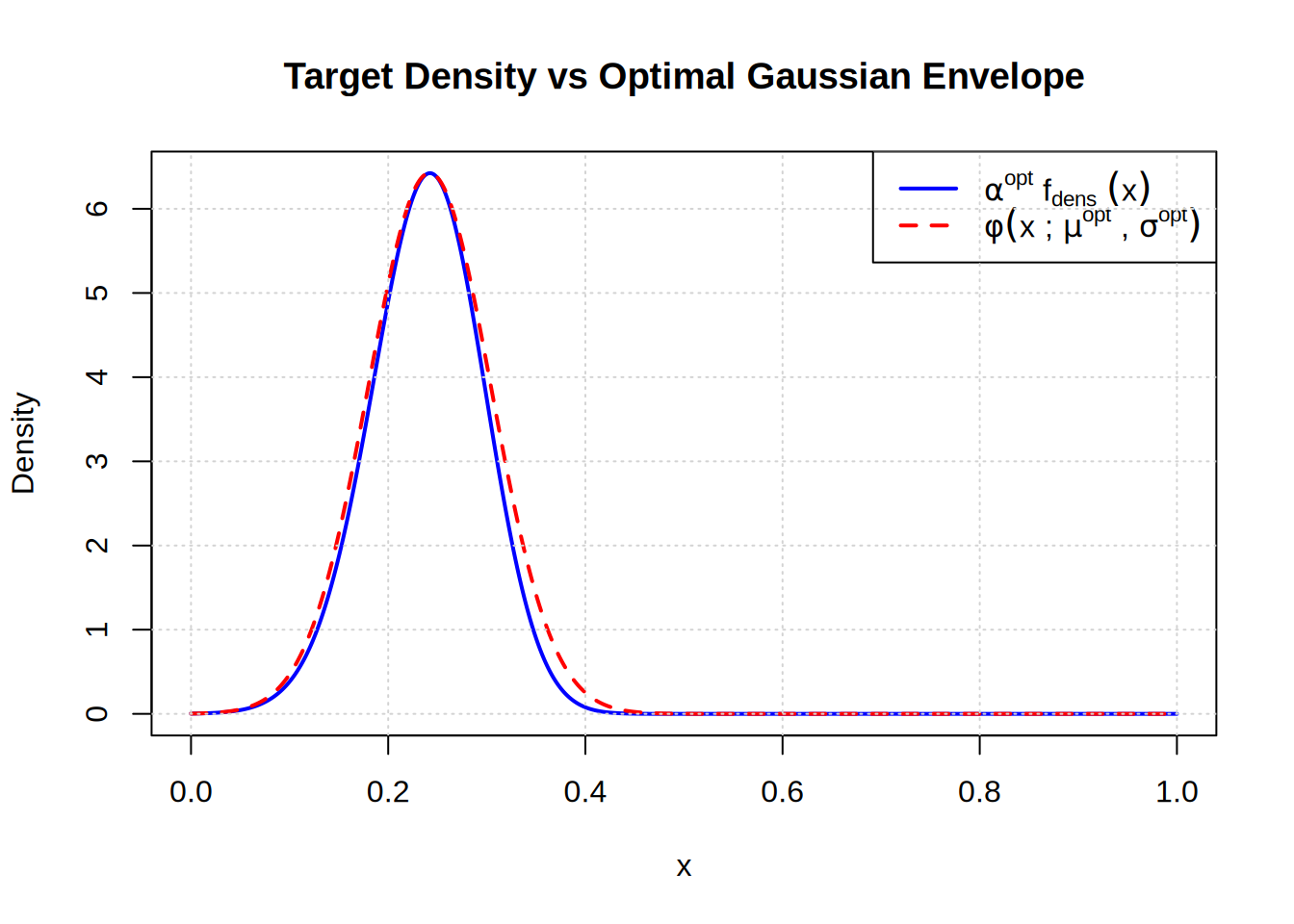
# Create the plot showing target density and optimal Gaussian envelopeplot(x_seq, f_dens1(x_seq, x, z) * alpha_opt,type ="l",lwd =2,col ="blue",ylab ="Density", xlab ="x",main ="Target Density vs Optimal Gaussian Envelope")# Add the optimal Gaussian envelopelines(x_seq, dnorm(x_seq, mu_opt, sd_opt), col ="red", lwd =2, lty =2)# Add legendlegend("topright", legend =c(expression(alpha^opt ~ f[dens] ~ (x)), expression(phi(x ~";"~ mu^opt ~","~ sigma^opt))), lty =c(1, 2), col =c("blue", "red"),lwd =2)# Add grid for better readabilitygrid()
This plot shows:
Blue line: The target density scaled by the optimal constant α^opt. This is the distribution we want to sample from.
Red dashed line: The optimal Gaussian envelope φ(x; μ^opt, σ^opt). This is what we use to generate candidate samples.
For rejection sampling to work properly, the proposal distribution must be greater than or equal to the target density everywhere. Here we see that:
μ^opt is the optimal mean that maximizes the target density
σ^opt is the optimal standard deviation that minimizes the rejection rate
α^opt is the optimal scaling constant that ensures the envelope covers the target
The optimization process finds the best Gaussian envelope that minimizes the rejection rate while ensuring the envelope properly covers the target density. This makes the rejection sampling as efficient as possible.
Let’s implement two versions of rejection sampling for a Poisson regression model:
#include <Rcpp.h>#include <random>usingnamespace Rcpp;// Target density: f(y) ∝ exp(y * sum(x*z) - sum(exp(y*x)))// Proposal: N(0,1) (standard normal)// Envelope: M * N(0,1) where M is chosen to bound f(y)// Branchy version - uses explicit if statement for acceptance/rejection// [[Rcpp::export]]NumericVector rejection_sampling_branchy(int n_samples,const NumericVector& x,const NumericVector& z,double alpha_log){ NumericVector samples(n_samples);std::mt19937 generator(std::random_device{}());std::normal_distribution<double> normal(0.0,1.0);std::uniform_real_distribution<double> uniform(0.0,1.0);int count =0;while(count < n_samples){double y_proposal = normal(generator);double u = uniform(generator);// Calculate log ratio: log(f(y)/g(y)) where g(y) is N(0,1)double sum_xz =0.0;double sum_exp =0.0;for(int i =0; i < x.size(); i++){ sum_xz += x[i]* z[i]; sum_exp += exp(y_proposal * x[i]);}double log_ratio = y_proposal * sum_xz - sum_exp +0.5* y_proposal * y_proposal;// Branch: accept or rejectif(log(u)<= alpha_log + log_ratio){ samples[count]= y_proposal; count++;}}return samples;}// Branchless version - uses arithmetic masking to avoid branching// [[Rcpp::export]]NumericVector rejection_sampling_branchless(int n_samples,const NumericVector& x,const NumericVector& z,double alpha_log){ NumericVector samples(n_samples);std::mt19937 generator(std::random_device{}());std::normal_distribution<double> normal(0.0,1.0);std::uniform_real_distribution<double> uniform(0.0,1.0);int count =0;while(count < n_samples){double y_proposal = normal(generator);double u = uniform(generator);// Calculate log ratio: log(f(y)/g(y)) where g(y) is N(0,1)double sum_xz =0.0;double sum_exp =0.0;for(int i =0; i < x.size(); i++){ sum_xz += x[i]* z[i]; sum_exp += exp(y_proposal * x[i]);}double log_ratio = y_proposal * sum_xz - sum_exp +0.5* y_proposal * y_proposal;// Branchless: use arithmetic to conditionally acceptdouble accept =(log(u)<= alpha_log + log_ratio); samples[count]= y_proposal * accept;// Only store if accepted, otherwise 0 count += accept;// Only increment if accepted}return samples;}
# Test both implementations using the optimal parameters from earlierset.seed(123)n_test <-5000# More samples for better timing# Use the optimal parameters calculated earliersamples_branchy <-rejection_sampling_branchy(n_test, x, z, mu_opt, sd_opt, alpha_opt)samples_branchless <-rejection_sampling_branchless(n_test, x, z, mu_opt, sd_opt, alpha_opt)# Compare results (first 10 samples)cat("Branchy version - first 10 samples:\n")
# Check that both methods produce similar resultscat("\nMean difference between methods:", mean(samples_branchy - samples_branchless), "\n")
Mean difference between methods: -4.041446e-05
cat("Max difference between methods:", max(abs(samples_branchy - samples_branchless)), "\n")
Max difference between methods: 0.3180189
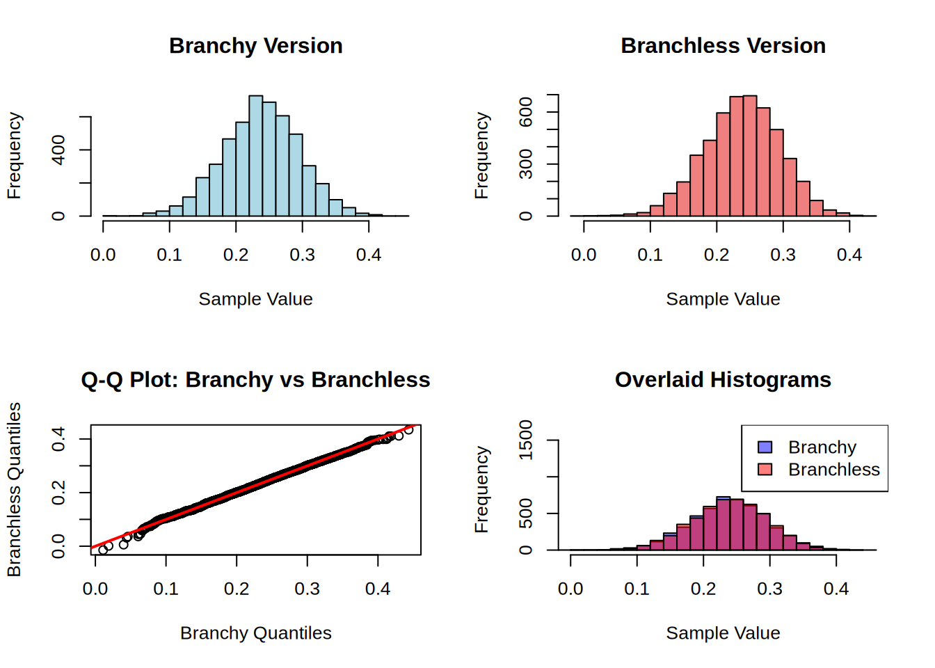
# Visual verification that both methods produce the same distributionpar(mfrow =c(2, 2))# Histogramshist(samples_branchy, breaks =30, main ="Branchy Version", xlab ="Sample Value", col ="lightblue", border ="black")hist(samples_branchless, breaks =30, main ="Branchless Version", xlab ="Sample Value", col ="lightcoral", border ="black")# Q-Q plot to compare distributionsqqplot(samples_branchy, samples_branchless, main ="Q-Q Plot: Branchy vs Branchless",xlab ="Branchy Quantiles", ylab ="Branchless Quantiles")abline(0, 1, col ="red", lwd =2) # Perfect correlation line# Overlaid histograms for direct comparisonhist(samples_branchy, breaks =30, main ="Overlaid Histograms", xlab ="Sample Value", col =rgb(0, 0, 1, 0.5), border ="black",ylim =c(0, max(c(hist(samples_branchy, plot =FALSE)$counts,hist(samples_branchless, plot =FALSE)$counts))))hist(samples_branchless, breaks =30, add =TRUE, col =rgb(1, 0, 0, 0.5), border ="black")legend("topright", legend =c("Branchy", "Branchless"), fill =c(rgb(0, 0, 1, 0.5), rgb(1, 0, 0, 0.5)))
par(mfrow =c(1, 1)) # Reset to single plot# Performance comparison with more iterationslibrary(bench)bench_results <- bench::mark(branchy =rejection_sampling_branchy(n_test, x, z, mu_opt, sd_opt, alpha_opt),branchless =rejection_sampling_branchless(n_test, x, z, mu_opt, sd_opt, alpha_opt),iterations =100, # More iterations for better statisticscheck =FALSE,min_time =1.0# Longer minimum time for more stable results)print(bench_results)
# A tibble: 2 × 13
  expression      min median `itr/sec` mem_alloc `gc/sec` n_itr  n_gc total_time
  <bch:expr> <bch:tm> <bch:>     <dbl> <bch:byt>    <dbl> <int> <dbl>   <bch:tm>
1 branchy      4.63ms 4.71ms      210.        NA        0   100     0      476ms
2 branchless   4.09ms 4.15ms      240.        NA        0   100     0      417ms
# ℹ 4 more variables: result <list>, memory <list>, time <list>, gc <list>
# Additional test with smaller sample sizecat("\n=== Testing with smaller sample size ===\n")
=== Testing with smaller sample size ===
# Test with smaller sample size to see if performance differences are consistentbench_small <- bench::mark(branchy_small =rejection_sampling_branchy(1000, x, z, mu_opt, sd_opt, alpha_opt),branchless_small =rejection_sampling_branchless(1000, x, z, mu_opt, sd_opt, alpha_opt),iterations =50,check =FALSE)print(bench_small)
# A tibble: 2 × 13
  expression      min median `itr/sec` mem_alloc `gc/sec` n_itr  n_gc total_time
  <bch:expr>    <bch> <bch:>     <dbl> <bch:byt>    <dbl> <int> <dbl>   <bch:tm>
1 branchy_small 926µs  952µs     1036.        NA        0    50     0     48.3ms
2 branchless_s… 816µs  838µs     1193.        NA        0    50     0     41.9ms
# ℹ 4 more variables: result <list>, memory <list>, time <list>, gc <list>
The key differences between the two approaches:
Branchy version: Uses an explicit if statement to decide whether to accept or reject each proposal. This creates a branch that the CPU must predict.
Branchless version: Uses arithmetic operations ((log(u) <= alpha_log + log_ratio)) to create a boolean mask, then uses this mask to conditionally increment the counter. This avoids the explicit branch.
In rejection sampling, the acceptance rate can vary significantly depending on how well the proposal distribution matches the target distribution. When the acceptance rate is low (many rejections), the branchy version may perform poorly due to branch mispredictions. The branchless version should be more consistent in performance regardless of the acceptance rate.
The branchless version correctly implements rejection sampling by using arithmetic operations instead of explicit branching. The count += accept line only increments the counter when accept = 1.0 (proposal accepted), and keeps it unchanged when accept = 0.0 (proposal rejected). This avoids the branch prediction overhead while maintaining the correct rejection sampling algorithm.