Solutions to Exercises Week 4

Keywords: currying, decorators, functional programming

Author

Jinyang Liu

Published

March 31, 2026

Exercise 25.2.6.1

Question: With the basics of C++ in hand, it’s now a great time to practice by reading and writing some simple C++ functions. For each of the following functions, read the code and figure out what the corresponding base R function is. You might not understand every part of the code yet, but you should be able to figure out the basics of what the function does.

cppFunction('
double f1(NumericVector x) {
  int n = x.size();
  double y = 0;

  for(int i = 0; i < n; ++i) {
    y += x[i] / n;
  }
  return y;
}
')

cppFunction('
NumericVector f2(NumericVector x) {
  int n = x.size();
  NumericVector out(n);

  out[0] = x[0];
  for(int i = 1; i < n; ++i) {
    out[i] = out[i - 1] + x[i];
  }
  return out;
}
')

cppFunction('
bool f3(LogicalVector x) {
  int n = x.size();
  bool any = false;
  for(int i = 0; i < n; ++i) {
    if (x[i]) any = true;
  }
  return any;
}
')

cppFunction('
int f4(Function pred, List x) {
  int n = x.size();

  for(int i = 0; i < n; ++i) {
    LogicalVector res = pred(x[i]);
    if (res[0]) return i + 1;
  }
  return 0;
}
')

cppFunction('
NumericVector f5(NumericVector x, NumericVector y) {
  int n = std::max(x.size(), y.size());
  NumericVector x1 = rep_len(x, n);
  NumericVector y1 = rep_len(y, n);

  NumericVector out(n);

  for (int i = 0; i < n; ++i) {
    out[i] = std::min(x1[i], y1[i]);
  }

  return out;
}
')

A: We can try running each function and seeing what they do. For example, we can run the following code:

x <- 1:4
f1(x) - mean(x) # f1 is the mean

[1] 0

f2(x) - cumsum(x) # f2 is the cumsum

[1] 0 0 0 0

f3(c(F, F, T, F)) == any(c(F, F, T, F)) # f3 is the any function

[1] TRUE

f4(function(x) c(x > 3, x > 6), 1:5) # finds the first in the list where the function has a truthy value

[1] 4

f5(1:5, 6:10) == apply(rbind(1:5, 6:10), MARGIN = 2, min) # f5 applies the min function to each column of the matrix

[1] TRUE TRUE TRUE TRUE TRUE

Exercise 25.2.6.2

To practice your function writing skills, convert the following functions into C++. For now, assume the inputs have no missing values. + all(). + cumprod(), cummin(), cummax(). + diff(). Start by assuming lag 1, and then generalise for lag n. + range(). + var(). Read about the approaches you can take on Wikipedia. Whenever implementing a numerical algorithm, it’s always good to check what is already known about the problem.

cppFunction('
bool all_cpp(LogicalVector x) {
  int n = x.size();
  for(int i = 0; i < n; ++i) {
    if (!x[i]) return false;
  }
  return true;
}
')

cppFunction('
double cumprod_cpp(NumericVector x) {
  int n = x.size();
  double prod = 1;

  for(int i = 0; i < n; ++i) {
    prod *= x[i];
  }
  return prod;
}
')

cppFunction('
NumericVector cummin_cpp(NumericVector x) {
  int n = x.size();
  double min = x[0];

  NumericVector out(n);
  out[0] = min;

  for(int i = 1; i < n; ++i) { // this is bad, why?
    if (x[i] < min) min = x[i];
    out[i] = min;
  }
  return out;
}
')

cppFunction('
NumericVector diff_cpp(NumericVector x, int lag = 1) {
  int n = x.size();
  NumericVector out(n - lag);

  for(int i = 0; i < n - lag; ++i) {
    out[i] = x[i + lag] - x[i];
  }
  return out;
}
')

cppFunction('
NumericVector range_cpp(NumericVector x) {
  double min = x[0], max = x[0];
  int n = x.size();

  for(int i = 1; i < n; ++i) {
    if (x[i] < min) min = x[i];
    if (x[i] > max) max = x[i];
  }

  NumericVector out = NumericVector::create(min, max);
  return out;
}
')

cppFunction('
double var_cpp(NumericVector x) {
  int n = x.size();
  double sum = 0, sumsq = 0;

  for(int i = 0; i < n; ++i) {
    sum += x[i];
    sumsq += x[i] * x[i];
  }

  return (sumsq - sum * sum / n) / (n - 1);
}
')

Question: See attached Rcpp file

all_cpp(c(F, T, T, T))

[1] FALSE

cumprod_cpp(1:5)

[1] 120

cummin_cpp(c(1, 2, 3, 0, 1))

[1] 1 1 1 0 0

diff_cpp(1:10, lag = 1)

[1] 1 1 1 1 1 1 1 1 1

diff_cpp(1:10, lag = 2)

[1] 2 2 2 2 2 2 2 2

range_cpp(1:10)

[1]  1 10

var_cpp(rnorm(1e5))

[1] 1.003504

Exercise 25.4.5.1

Question: Rewrite any of the functions from the first exercise of Section 25.2.6 to deal with missing values. If na.rm is true, ignore the missing values. If na.rm is false, return a missing value if the input contains any missing values. Some good functions to practice with are min(), max(), range(), mean(), and var().

Answer: Use the decorator design pattern,

.na.rm_decorator <- function(fun) {
  function(x, na.rm = FALSE, ...) {
    if (na.rm) {
      x <- x[!is.na(x)]
    } else if (any(is.na(x))) {
      return(NA)
    }
    return(fun(x, ...))
  }
}

## shorter version using only one if statement
.na.rm_decorator_2 <- function(fun) {
  function(x, na.rm = FALSE, ...) {
    if (!na.rm && any(is.na(x))) {
      return(NA)
    }
    x <- x[!is.na(x)]
    return(fun(x, ...))
  }
}

Use our decorators

mean_decorated <- .na.rm_decorator(f1)

mean_decorated(c(1, 2, NA, 3, 4))

[1] NA

mean_decorated(c(1, 2, NA, 3, 4), na.rm = TRUE)

[1] 2.5

mean_decorated(c(1, 2, 3, 4))

[1] 2.5

diff_decorated <- .na.rm_decorator_2(diff_cpp)
diff_decorated(c(1, 2, NA, 3, 4), lag = 2)

[1] NA

diff_decorated(c(1, 2, NA, 3, 4), na.rm = TRUE, lag = 2)

[1] 2 2

diff_decorated(c(1, 2, 3, 4), lag = 2)

[1] 2 2

Exercise 25.4.5.2

Question: Rewrite cumsum() and diff() so they can handle missing values. Note that these functions have slightly more complicated behaviour.

Answer: Use the decorator pattern again.

# For cumsum: use the first decorator (treats NAs as 0 when na.rm = TRUE)
cumsum_decorated <- .na.rm_decorator(f2)

# For diff: use the second decorator (removes NAs when na.rm = TRUE)
diff_decorated <- .na.rm_decorator_2(diff_cpp)

# Test the decorated functions
test_vec <- c(1, 2, NA, 4, 5)

# Test cumsum
cumsum_decorated(test_vec, na.rm = FALSE)  # Should return NAs

[1] NA

cumsum_decorated(test_vec, na.rm = TRUE)   # Should treat NA as 0

[1]  1  3  7 12

# Test diff  
diff_decorated(test_vec, lag = 1, na.rm = FALSE)  # Should return NAs

[1] NA

diff_decorated(test_vec, lag = 1, na.rm = TRUE)   # Should work on non-NA values

[1] 1 2 1

Bonus Example: Currying with Kernel Density Estimation (AI generated)

Question: How can we use currying (function composition and partial application) to create flexible and reusable kernel density estimation functions?

A: In U2.qmd, we implemented kernel density estimation with the Epanechnikov kernel. Now let’s see how currying can make our code more modular and elegant.

Step 1: Define Different Kernel Functions

First, let’s define several kernel functions:

# Epanechnikov kernel (from U2.qmd)
epanechnikov_kernel <- function(z) (abs(z) <= 1) * (1 - z^2) * 3 / 4 

# Gaussian kernel
gaussian_kernel <- function(z) (1 / sqrt(2 * pi)) * exp(-0.5 * z^2)

# Uniform kernel
uniform_kernel <- function(z) (abs(z) <= 1) * 0.5

# Triangular kernel
triangular_kernel <- function(z) (abs(z) <= 1) * (1 - abs(z))

Step 2: Create a General Kernel Density Function

Now let’s create a general function that can work with any kernel:

# General kernel density estimation function
kern_dens_general <- function(x, h, kernel_func, n = 512) {
  rg <- range(x)
  xx <- seq(rg[1] - 3 * h, rg[2] + 3 * h, length.out = n)
  y <- numeric(n)
  
  for (i in seq_along(xx)) {
    y[i] <- mean(kernel_func((xx[i] - x) / h)) / h
  }
  list(x = xx, y = y)
}

Step 3: Using Currying to Create Specialized Functions

Now comes the magic of currying! We can create specialized functions by “currying” our general function:

# Curry by kernel type - creates functions that use specific kernels
epanechnikov_kde <- function(x, h, n = 512) kern_dens_general(x, h, epanechnikov_kernel, n)

gaussian_kde <- function(x, h, n = 512) kern_dens_general(x, h, gaussian_kernel, n)

uniform_kde <- function(x, h, n = 512) kern_dens_general(x, h, uniform_kernel, n)

# Curry by bandwidth - creates functions with fixed bandwidths
epanechnikov_bw_half <- function(x, n = 512) epanechnikov_kde(x, h = 0.5, n)

epanechnikov_bw_one <- function(x, n = 512) epanechnikov_kde(x, h = 1.0, n)

epanechnikov_bw_two <- function(x, n = 512) epanechnikov_kde(x, h = 2.0, n)

Step 4: Advanced Currying - Function Factories

We can create “function factories” that generate curried functions:

# Factory function that creates kernel-specific KDE functions
make_kernel_kde <- function(kernel_func) {
  function(x, h, n = 512) kern_dens_general(x, h, kernel_func, n)
}

# Factory function that creates bandwidth-specific functions
make_bandwidth_kde <- function(kde_func, bandwidth) {
  function(x, n = 512) kde_func(x, h = bandwidth, n)
}

# Create kernel-specific functions using the factory
epa_kde <- make_kernel_kde(epanechnikov_kernel)
gauss_kde <- make_kernel_kde(gaussian_kernel)

# Create bandwidth-specific functions
epa_narrow <- make_bandwidth_kde(epa_kde, 0.3)
epa_medium <- make_bandwidth_kde(epa_kde, 0.8)
epa_wide <- make_bandwidth_kde(epa_kde, 1.5)

Step 5: Demonstration with Data

Let’s test our curried functions with the infrared data:

# Load the data (same as U2.qmd)
infrared <- read.table(here::here("data", "infrared.txt"), header = TRUE)
F12 <- infrared$F12
log_F12 <- log(F12)

# Test our curried functions
dens_narrow <- epa_narrow(log_F12)
dens_medium <- epa_medium(log_F12)
dens_wide <- epa_wide(log_F12)

# Compare different kernels with same bandwidth
dens_epa <- epa_kde(log_F12, h = 0.8)
dens_gauss <- gauss_kde(log_F12, h = 0.8)
dens_uniform <- make_kernel_kde(uniform_kernel)(log_F12, h = 0.8)

Step 6: Visualization

library(ggplot2)

# Create data frames for plotting
df_bandwidths <- data.frame(
  x = rep(dens_narrow$x, 3),
  y = c(dens_narrow$y, dens_medium$y, dens_wide$y),
  bandwidth = rep(c("Narrow (0.3)", "Medium (0.8)", "Wide (1.5)"), each = length(dens_narrow$x))
)

df_kernels <- data.frame(
  x = rep(dens_epa$x, 3),
  y = c(dens_epa$y, dens_gauss$y, dens_uniform$y),
  kernel = rep(c("Epanechnikov", "Gaussian", "Uniform"), each = length(dens_epa$x))
)

# Plot different bandwidths
p1 <- ggplot(df_bandwidths, aes(x = x, y = y, color = bandwidth)) +
  geom_line(size = 1) +
  labs(title = "Effect of Bandwidth (Epanechnikov Kernel)",
       x = "log(F12)", y = "Density", color = "Bandwidth") +
  theme_minimal()

# Plot different kernels
p2 <- ggplot(df_kernels, aes(x = x, y = y, color = kernel)) +
  geom_line(size = 1) +
  labs(title = "Different Kernels (h = 0.8)",
       x = "log(F12)", y = "Density", color = "Kernel") +
  theme_minimal()

print(p1)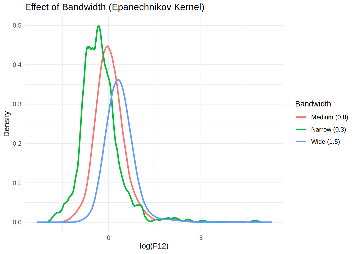

print(p2)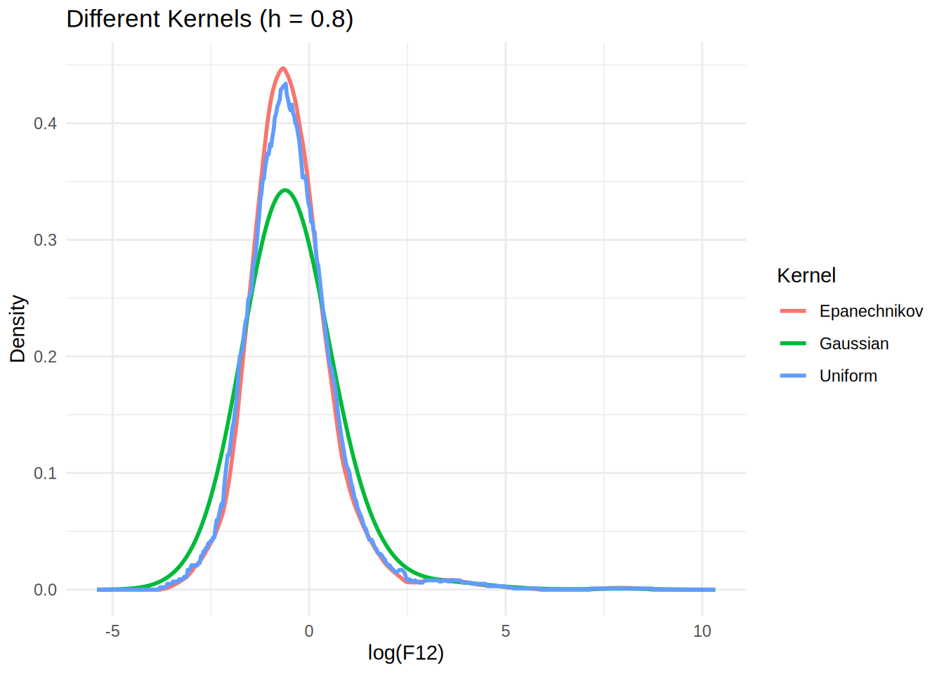

Key Benefits of This Currying Approach:

Modularity: Each component (kernel, bandwidth) can be modified independently
Reusability: Once created, curried functions can be reused multiple times
Readability: Code becomes more self-documenting (e.g., epa_narrow clearly indicates both kernel and bandwidth)
Flexibility: Easy to create new combinations without rewriting core logic
Functional Programming: Demonstrates higher-order functions and partial application

Advanced Example: Pipeline Processing

# Create a pipeline for comparing multiple bandwidth settings
bandwidth_comparison <- function(data, bandwidths) {
  kde_functions <- lapply(bandwidths, function(bw) {
    make_bandwidth_kde(epa_kde, bw)
  })
  
  results <- lapply(kde_functions, function(f) f(data))
  names(results) <- paste("bw", bandwidths, sep = "_")
  return(results)
}

# Use the pipeline
comparison_results <- bandwidth_comparison(log_F12, c(0.2, 0.5, 1.0, 1.5))

# Each result is readily available
str(comparison_results$bw_0.5, max.level = 1)

List of 2
 $ x: num [1:512] -4.5 -4.47 -4.44 -4.41 -4.39 ...
 $ y: num [1:512] 0 0 0 0 0 0 0 0 0 0 ...

str(comparison_results$bw_1.0, max.level = 1)

 NULL

str(comparison_results$bw_1.5, max.level = 1)

List of 2
 $ x: num [1:512] -7.5 -7.46 -7.42 -7.38 -7.34 ...
 $ y: num [1:512] 0 0 0 0 0 0 0 0 0 0 ...

This example shows how currying transforms our kernel density estimation from a monolithic function into a flexible, composable system. It’s the same principle we used with the .na.rm_decorator - we’re creating specialized functions from more general ones!