infrared <- read.table(here::here("data", "infrared.txt"), header = TRUE)
F12 <- infrared$F12Solutions to Exercises Week 2
Keywords: KDE, benchmarking, memory usage
Exercise 2.1
Q: The Epanechnikov kernel is given by
K(x)= \begin{cases}\frac{3}{4}\left(1-x^2\right), & \text { if } x \in[-1,1] \\ 0, & \text { otherwise }\end{cases}
Show that this is a probability density with mean zero and compute \sigma_K^2 and \|K\|_2^2 as defined in CSWR paragraph 2.3.2.
Solution: Since K is non-negative, integrable, and integrates to one over the entire sample space,
\int_{\mathbb{R}} \frac{3}{4}\left(1-x^2\right) \mathbf{1}_{[-1,1]}(x) \mathrm{d} x=\frac{3}{4} \int_{-1}^1\left(1-x^2\right) \mathrm{d} x=\frac{3}{4}\left[x-\frac{1}{3} x^3\right]_{-1}^1=1
K is a probability density function. For an absolutely continuous random variable X with density K we have the following properties:
\begin{aligned} \mathbb{E}[X] & =\int_{\mathbb{R}} x K(x) \mathrm{d} x=\frac{3}{4} \int_{-1}^1\left(x-x^3\right) \mathrm{d} x=\frac{3}{4}\left[\frac{1}{2} x^2-\frac{1}{4} x^4\right]_{-1}^1=0 \\ \sigma_K^2 & =\mathbb{E}\left[X^2\right]=\int_{\mathbb{R}} x^2 K(x) \mathrm{d} x=\frac{3}{4} \int_{-1}^1\left(x^2-x^4\right) \mathrm{d} x=\frac{3}{4}\left[\frac{1}{3} x^3-\frac{1}{5} x^5\right]_{-1}^1=\frac{1}{5} \\ \mathbb{V}[X] & =\mathbb{E}\left[X^2\right]-\mathbb{E}[X]^2=\frac{1}{5} \\ \|K\|_2^2 & =\int_{\mathbb{R}} K^2(x) \mathrm{d} x=\frac{9}{16} \int_{-1}^1\left(1+x^4-2 x^2\right) \mathrm{d} x=\frac{9}{16}\left[x+\frac{1}{5} x^5-\frac{2}{3} x^3\right]_{-1}^1=\frac{3}{5} \end{aligned}
Take away points: The properties of many kernels are completely known. If you want an implementation to take different default kernels as input, you can store such information in a list that is accessible for your functions. That way your implementation saves a lot of calculation. If you want your implementation to take any probability density as input, then you need a smart way to calculate the above quantities.
Exercise 2.2
Q: Use density() to compute the kernel density estimate with the Epanechnikov kernel to the log(F12) data. Try different bandwidths.
A: Download the infrared data set from this link and place it in the data/ folder of your working directory. Then load the data:
We can compute the density estimates as follows with bw = 1
dens <- density(log(F12), bw = 1, kernel = "epanechnikov")Plot the density using ggplot, here we can use stat_density or plot it the old way
dens_df <- as.data.frame(dens[1:2])
p0 <- ggplot(infrared, aes(x = log(F12))) +
  stat_density(kernel = "epanechnikov", bw = 1, fill = "green")

p1 <- ggplot(infrared, aes(x = log(F12), y = after_stat(density))) +
   geom_histogram(bins = 20, fill = "blue", alpha = 0.3) +
   geom_line(data = dens_df, aes(x = x, y = y), color = "red") +
   xlim(-4, 12) +
   ylim(0, 0.6)

p0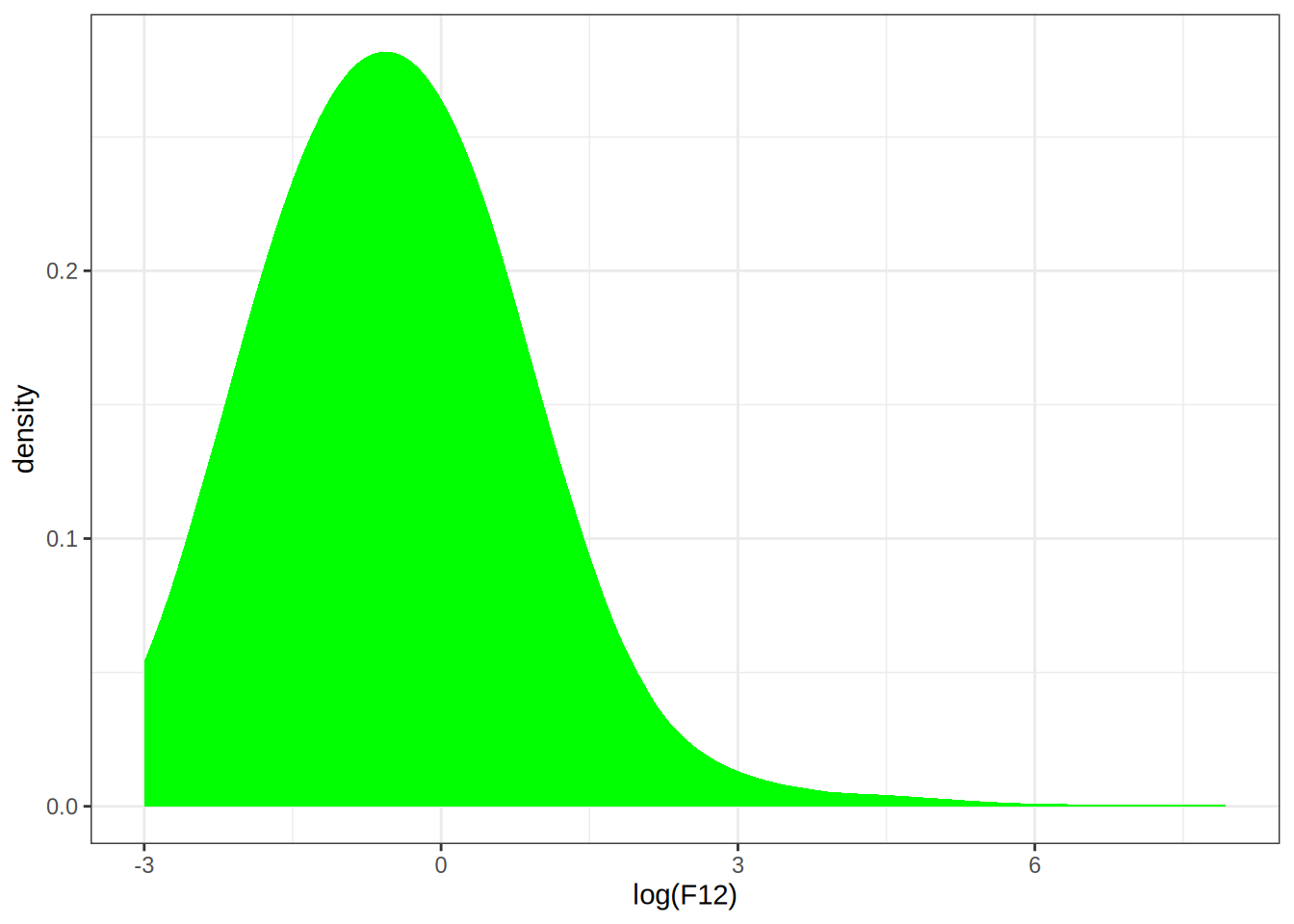
p1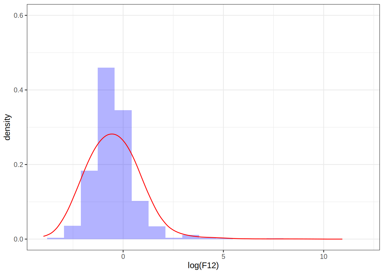
Setting the bandwidth to 0.1
# Density estimates with bw = 0.1
dens <- as.data.frame(density(log(F12), bw = 0.1, kernel = "epanechnikov")[1:2])
p <- p1 + geom_line(data = dens, aes(x = x, y = y), color = "purple")
p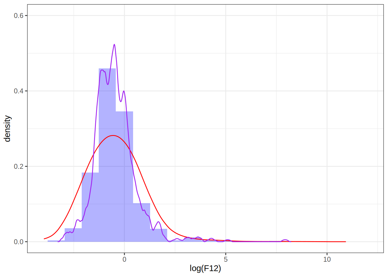
Setting the bandwidth to 0.5
dens <- as.data.frame(density(log(F12), bw = 0.5, kernel = "epanechnikov")[1:2])
p <- p + geom_line(data = dens, aes(x = x, y = y), color = "blue")
p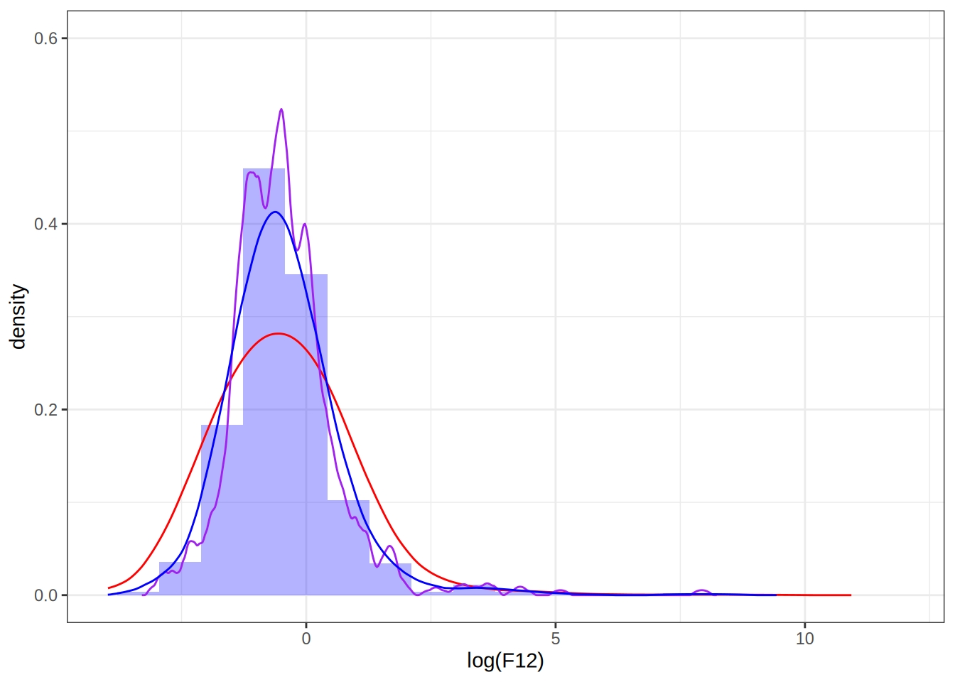
Take away points: bandwidth selection determines how well the density estimate fits the data, choosing it too small can result in overfitting.
Exercise 2.3
Q: Implement kernel density estimation yourself using the Epanechnikov kernel. Test your implementation by comparing it to density() using the log(F12) data.
A: Modify the existing function from the book
# FALSE * number == 0
kern <- function(z) (abs(z) <= 1) * (1 - z^2) * 3 / 4

kern_dens_vec <- function(x, h, n = 512) {
  rg <- range(x)
  xx <- seq(rg[1] - 3 * h, rg[2] + 3 * h, length.out = n)
  y <- numeric(n)
  # The inner loop from 'kern_dens_loop()' has been vectorized, and
  # only the outer loop over the grid points remains.
  for (i in seq_along(xx)) {
      y[i] <- mean(kern((xx[i] - x)/h)) /h
  }
  list(x = xx, y = y)
}
Compare it with density
my_dens_df <- as.data.frame(kern_dens_vec(log(F12), 1)[1:2])
p1 + geom_line(data = my_dens_df, aes(x = x, y = y), color = "green")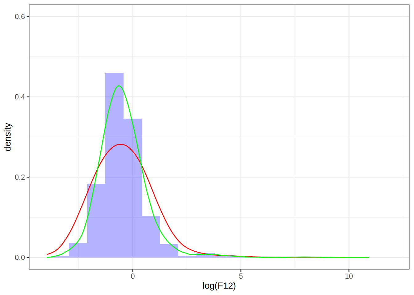
The two estimates don’t match, despite the bandwidths being the same, why is that? If we look at the documentation for density(), we see that it uses a normalized kernel that guarantees \sigma_K^2 is scaled to 1. That means that the bandwidth we set on our kernel will have a different effect than setting the bandwidth on density(), luckily, we can scale our bandwidth by a factor in order to obtain the same density estimate as we would have gotten by using density(). Namely, if we set the bandwidth to be h = 1 in density(), then we can choose our bandwidth to be \tilde{h} = (\sigma_K^2)^{-1/2} h= (1/5)^{-1/2} to get the same density estimate, see this article.
my_dens_df2 <- as.data.frame(kern_dens_vec(log(F12), sqrt(5))[1:2])
p1 + geom_line(data = my_dens_df2, aes(x = x, y = y), color = "green", alpha = 0.5)
Exercise 2.4
Q: Construct the following vector
x <- rnorm(2^13)Then use bench::mark() to benchmark the computation of
density(x[1:k], 0.2)for k ranging from 2^5 to 2^{13}. Summarize the benchmarking results.
A: Ok let’s do the following
# Load necessary libraries
library(bench)

# Construct the vector
x <- rnorm(2^13)

benchmark_results <- bench::press(
  k = 2^(5:13),
  {
    bench::mark(
      density(x[1:k], 0.2),
      check = F
    )
  }
)
Running with:
k1 322 643 1284 2565 5126 10247 20488 40969 8192# Summarize the benchmarking results
autoplot(benchmark_results)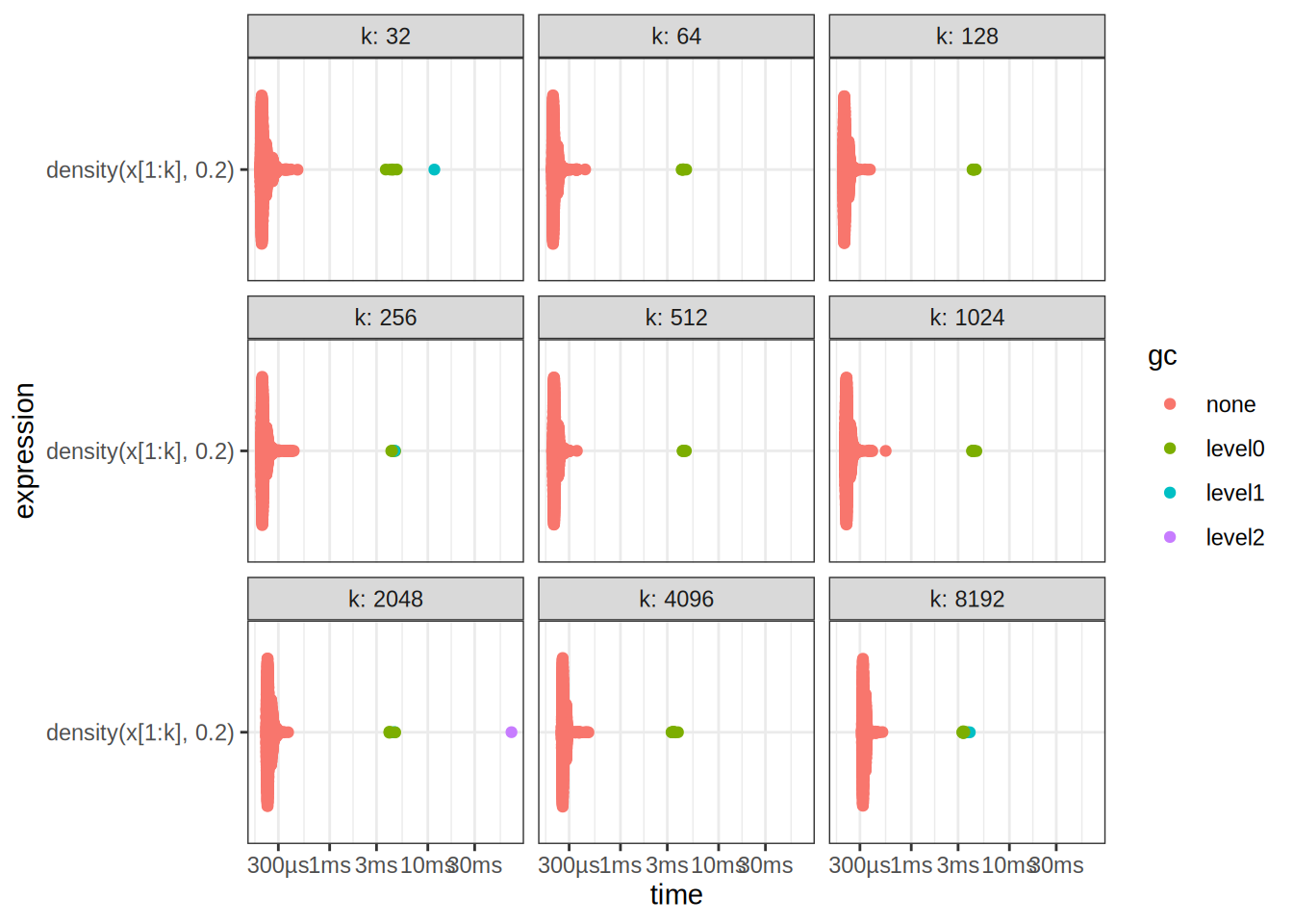
benchmark_results# A tibble: 9 × 7
expression k min median `itr/sec` mem_alloc `gc/sec`
<bch:expr> <dbl> <bch:tm> <bch:tm> <dbl> <bch:byt> <dbl>
1 density(x[1:k], 0.2) 32 195µs 209µs 4557. NA 12.9
2 density(x[1:k], 0.2) 64 198µs 210µs 4615. NA 14.9
3 density(x[1:k], 0.2) 128 201µs 212µs 4594. NA 12.7
4 density(x[1:k], 0.2) 256 199µs 210µs 4581. NA 14.9
5 density(x[1:k], 0.2) 512 200µs 214µs 4536. NA 12.7
6 density(x[1:k], 0.2) 1024 210µs 222µs 4362. NA 14.9
7 density(x[1:k], 0.2) 2048 224µs 238µs 4082. NA 17.4
8 density(x[1:k], 0.2) 4096 250µs 261µs 3738. NA 19.2
9 density(x[1:k], 0.2) 8192 312µs 327µs 3004. NA 23.8Exercise 2.5
Q: Benchmark your own implementation of kernel density estimation using the Epanechnikov kernel. Compare the results to those obtained for density().
A: If we look at our own results, we observe that the benchmark times are scattered with a higher variance, and after k = 2^{11} points, we begin calling the garbage collector in pretty much all of the cases.
benchmark_results2 <- bench::press(
  k = 2^(5:13),
  {
    bench::mark(
      kern_dens_vec(x[1:k], 0.2),
      check = F
    )
  }
)
Running with:
k1 322 643 1284 2565 5126 10247 20488 4096Warning: Some expressions had a GC in every iteration; so filtering is
disabled.9 8192Warning: Some expressions had a GC in every iteration; so filtering is
disabled.autoplot(benchmark_results2)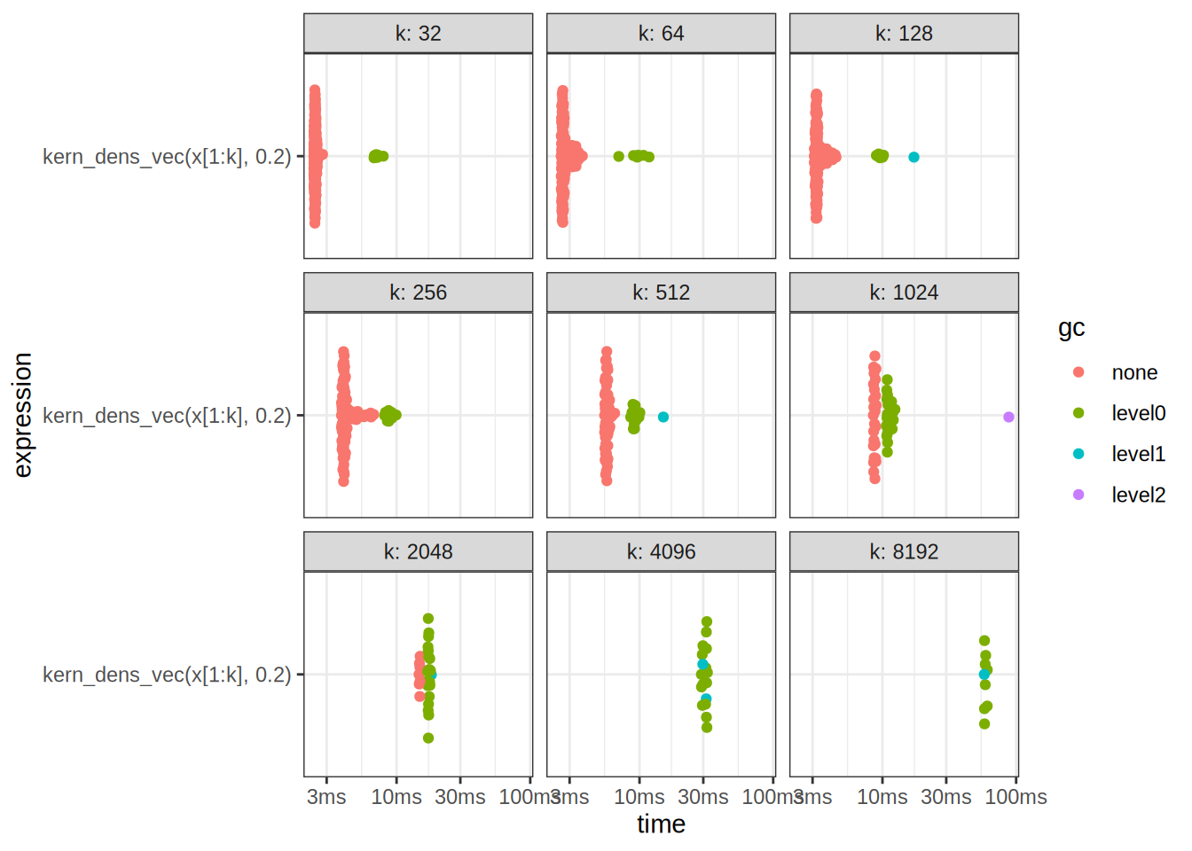
print(benchmark_results2)# A tibble: 9 × 14
expression k min median `itr/sec` mem_alloc `gc/sec` n_itr n_gc
<bch:expr> <dbl> <bch:t> <bch:t> <dbl> <bch:byt> <dbl> <int> <dbl>
1 kern_dens_vec(… 32 2.4ms 2.46ms 405. NA 15.5 183 7
2 kern_dens_vec(… 64 2.59ms 2.69ms 354. NA 16.2 153 7
3 kern_dens_vec(… 128 3.09ms 3.23ms 298. NA 19.2 124 8
4 kern_dens_vec(… 256 3.87ms 4.06ms 234. NA 30.1 93 12
5 kern_dens_vec(… 512 5.48ms 5.68ms 175. NA 50.4 59 17
6 kern_dens_vec(… 1024 8.55ms 8.7ms 115. NA 87.1 25 19
7 kern_dens_vec(… 2048 14.72ms 14.92ms 67.2 NA 221. 7 23
8 kern_dens_vec(… 4096 29.03ms 31.38ms 32.5 NA 51.6 17 27
9 kern_dens_vec(… 8192 57.77ms 58.7ms 17.0 NA 54.7 9 29
# ℹ 5 more variables: total_time <bch:tm>, result <list>, memory <list>,
# time <list>, gc <list>We can also look at the time complexities of both methods
# Extract median times from benchmark results
median_times_density <- summary(benchmark_results)$median
median_times_kern_dens_vec <- summary(benchmark_results2)$median
Warning: Some expressions had a GC in every iteration; so filtering is
disabled.# Create a data frame for plotting
input_sizes <- 2^(5:13)
benchmark_data <- data.frame(
InputSize = rep(input_sizes, 2),
MedianTime = c(median_times_density, median_times_kern_dens_vec),
Method = rep(c("density", "kern_dens_vec"), each = length(input_sizes))
)
# Plot the median times against input sizes
ggplot(benchmark_data, aes(x = InputSize, y = MedianTime, color = Method)) +
geom_line() +
geom_point() +
scale_y_continuous(trans = 'log2') +
scale_x_continuous(trans = 'log2') +
labs(title = "Median Times vs Input Sizes",
x = "Input Size (log2 scale)",
y = "Median Time (log2 scale)",
color = "Method") +
theme_minimal()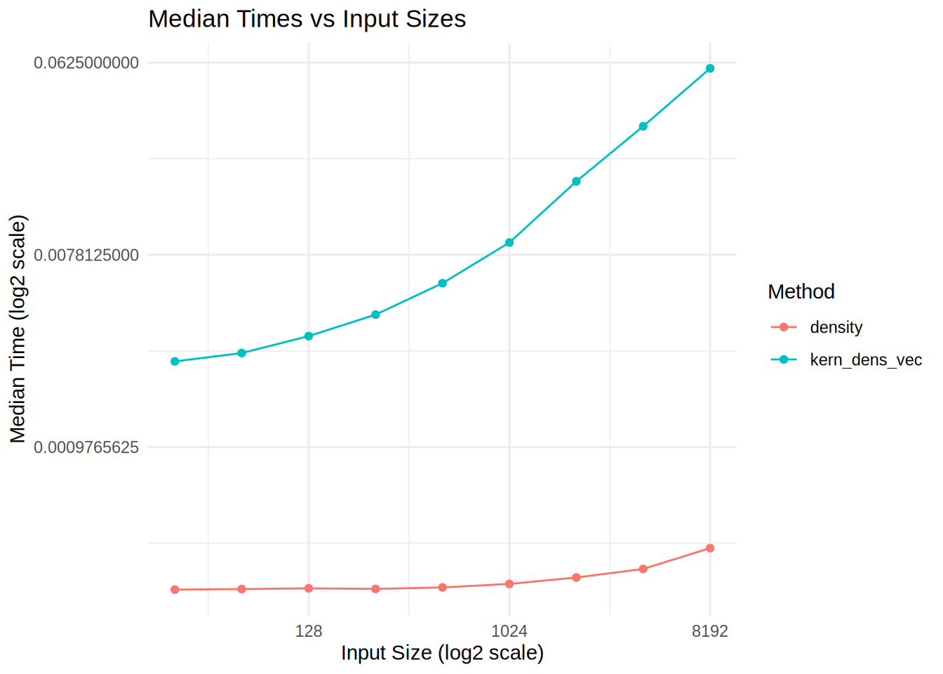
We see that our kernel estimate has a different time complexity, it also uses more memory, what can we do to optimize it?
Exercise 2.6
You have all the tools you need to solve this by yourself! Remember, programming is a craftsmanship, so try different things out to see what works and doesn’t.
Exercise 24.4.3.2 (interesting)
Q: Make a faster version of chisq.test() that only computes the chi-square test statistic when the input is two numeric vectors with no missing values. You can try simplifying chisq.test() or by coding from the mathematical definition.
A: Okay, we will try:
x <- sample(1:3, 100, replace = T)
y <- sample(4:5, 100, replace = T)

chisq_test_improved <- function(x, y, tab_fun = table) {
  M <- tab_fun(x, y)
  m_i <- rowSums(M) %o% colSums(M) / sum(M)

  sum((M - m_i)^2 / m_i)
}

chisq_test_improved(x, y)
[1] 1.264917chisq.test(x, y)$statisticX-squared
1.264917 NB: notice in the implementation above, we pass in the table function as an argument. This is a versatile design pattern known as Dependency Injection, and can be used to switch the behavior of a function during Runtime. In contrast, imagine hardcoding the table function into the implementation, we would have to change the implementation if we wanted to use a different table function.
We can now benchmark the two, seems that our implementation is fast!
res <- bench::mark(
  chisq_test_improved(x, y),
  chisq.test(x, y)$statistic,
  check = F
)

autoplot(res)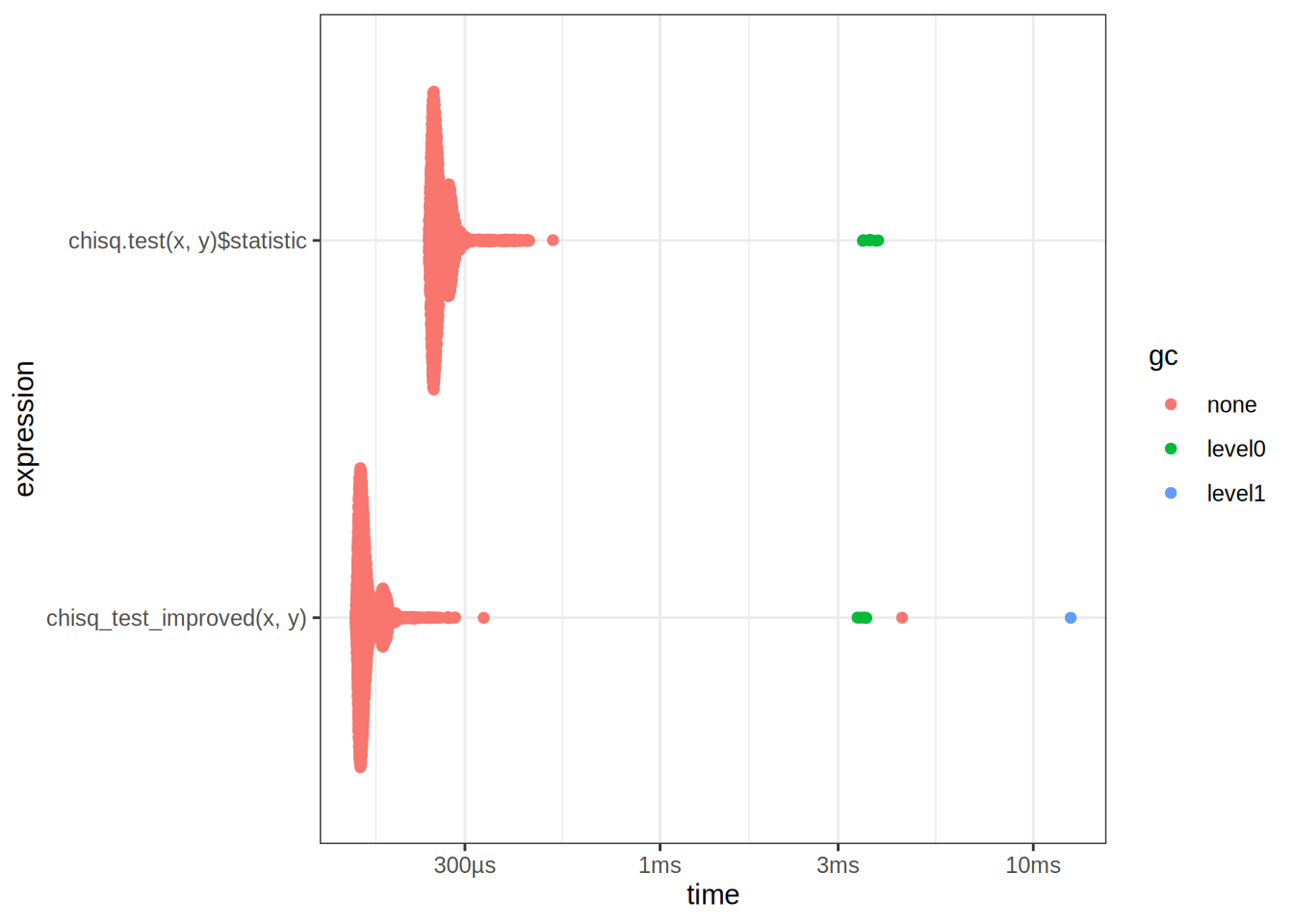
res# A tibble: 2 × 6
expression min median `itr/sec` mem_alloc `gc/sec`
<bch:expr> <bch:tm> <bch:tm> <dbl> <bch:byt> <dbl>
1 chisq_test_improved(x, y) 153µs 160µs 6009. NA 10.6
2 chisq.test(x, y)$statistic 240µs 253µs 3833. NA 12.5Exercise 24.4.3.3 (interesting)
Q: Can you make a faster version of table() for the case of an input of two integer vectors with no missing values? Can you use it to speed up your chi-square test?
A: Let’s try the following:
fast_table <- function(x, y) {
  unique_x <- sort(unique(x))
  unique_y <- sort(unique(y))

  table_matrix <- matrix(0, nrow = length(unique_x), ncol = length(unique_y))
  rownames(table_matrix) <- unique_x
  colnames(table_matrix) <- unique_y

  for (i in unique_x) {
    for (j in unique_y) {
      table_matrix[as.character(i), as.character(j)] <- sum(x == i & y == j)
    }
  }

  table_matrix
}
fast_table(x,y)
4 5
1 14 18
2 13 26
3 9 20table(x,y) y
x 4 5
1 14 18
2 13 26
3 9 20Benchmark it to see if it is really faster:
table_bench <- bench::mark(
  table(x, y),
  fast_table(x,y),
  check = F
)
autoplot(table_bench)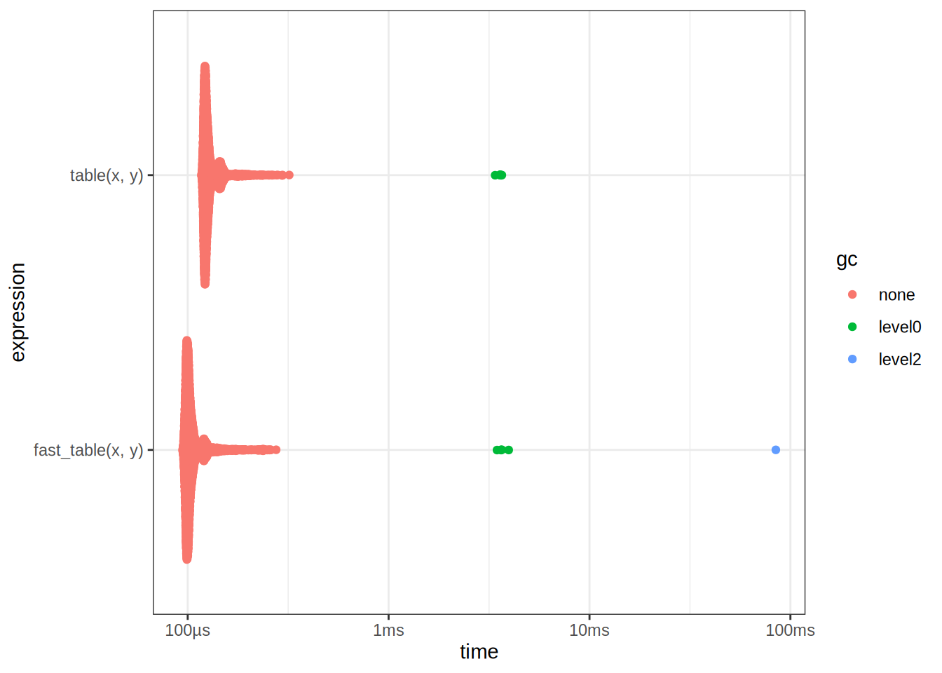
table_bench# A tibble: 2 × 6
expression min median `itr/sec` mem_alloc `gc/sec`
<bch:expr> <bch:tm> <bch:tm> <dbl> <bch:byt> <dbl>
1 table(x, y) 117µs 124µs 7715. NA 12.5
2 fast_table(x, y) 94.2µs 101µs 9366. NA 14.3We see that it is faster, this is really because table does a lot of different things under the hood, validating inputs etc. If we can guarantee that the inputs are correct, then we can drop the extra validation steps to obtain a speedup. But wait, we can make it even faster?
fast_table2 <- function(x, y) {
  fx <- as.factor(x)
  fy <- as.factor(y)
  lx <- levels(fx)
  ly <- levels(fy)

  pd <- 1
  bin <- 0L
  bin <- bin + pd * (as.integer(fx) - 1L)
  pd <- pd * length(lx)

  bin <- bin + pd * (as.integer(fy) - 1L)
  pd <- pd * length(ly)

  array(tabulate(bin + 1, pd), c(length(lx), length(ly)), dimnames = list(lx, ly))
}
Benchmark it:
table_bench2 <- bench::mark(
  table(x, y),
  fast_table(x,y),
  fast_table2(x,y),
  check = F
)
autoplot(table_bench2)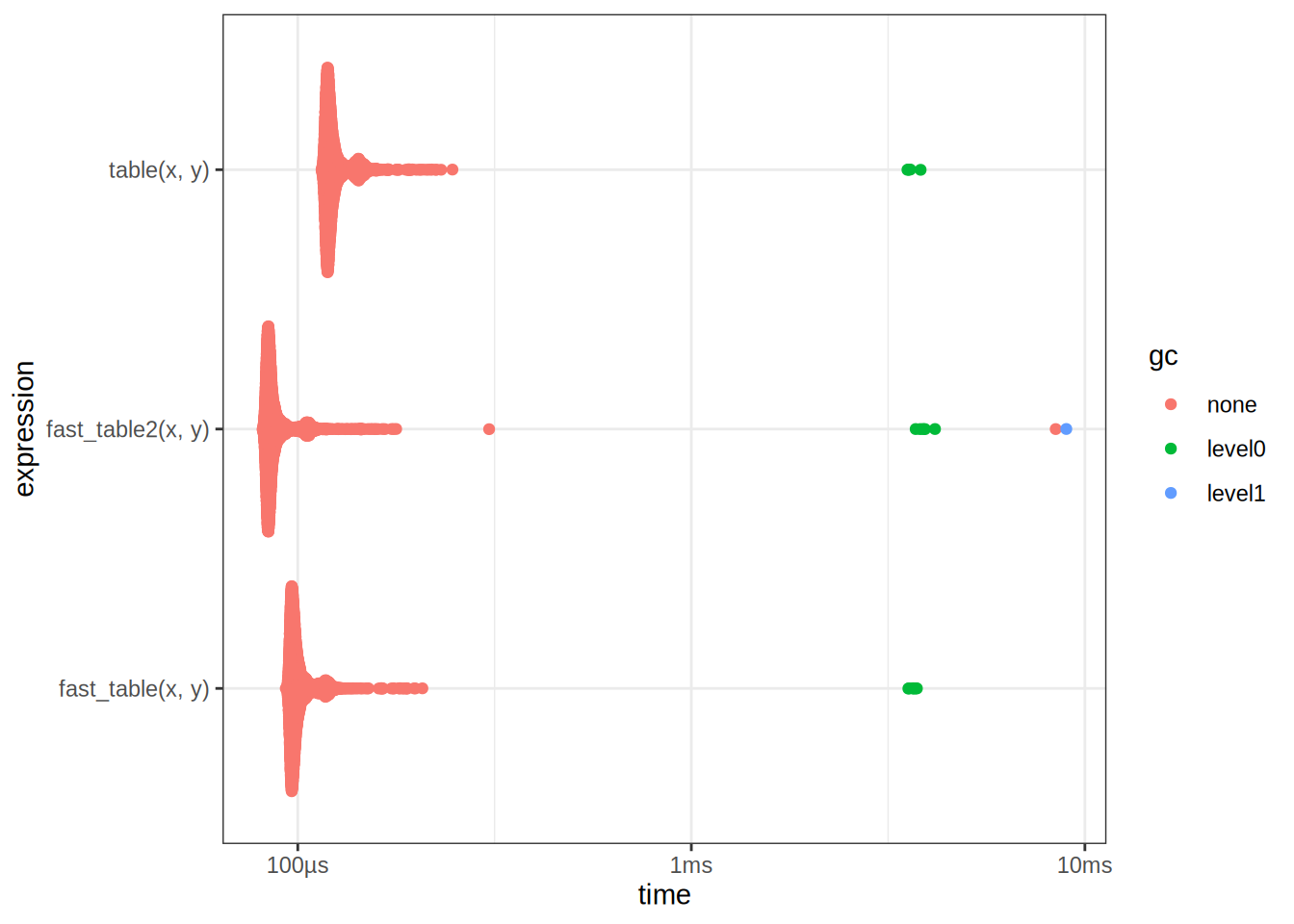
table_bench# A tibble: 2 × 6
expression min median `itr/sec` mem_alloc `gc/sec`
<bch:expr> <bch:tm> <bch:tm> <dbl> <bch:byt> <dbl>
1 table(x, y) 117µs 124µs 7715. NA 12.5
2 fast_table(x, y) 94.2µs 101µs 9366. NA 14.3We see that it is faster! However I did not come up with this implementation myself, nor did I ask AI. I simply reversed engineered it from the implementation of table. One can inspect the source code by typing table in the R console. To reverse engineer code by hand, it is often beneficial to use a debugger, and step through the code line by line. We can now optimize our ChiSq test using this new implementation:
chisq_bench <- bench::mark(
  chisq_test_improved(x, y, tab_fun = table),
  chisq_test_improved(x, y, tab_fun = fast_table),
  chisq_test_improved(x, y, tab_fun = fast_table2)
)
autoplot(chisq_bench)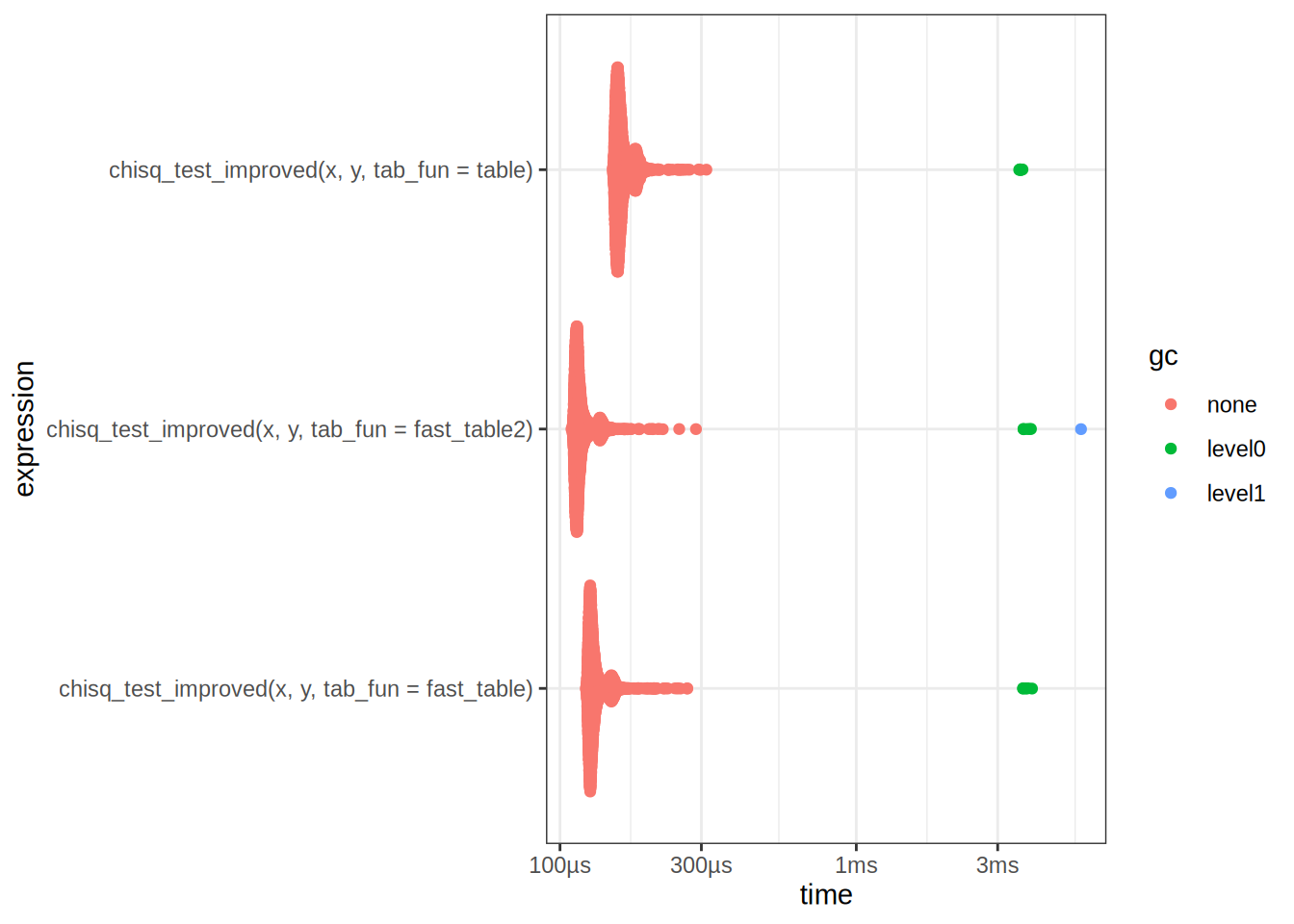
chisq_bench# A tibble: 3 × 6
expression min median `itr/sec` mem_alloc `gc/sec`
<bch:expr> <bch> <bch:> <dbl> <bch:byt> <dbl>
1 chisq_test_improved(x, y, tab_fun =… 151µs 159µs 6122. NA 12.5
2 chisq_test_improved(x, y, tab_fun =… 122µs 128µs 7544. NA 12.6
3 chisq_test_improved(x, y, tab_fun =… 109µs 115µs 8419. NA 12.6Take away points: There are many different ways to optimize code, a common strategy is to break down the problem into smaller subproblems, and then optimize each subproblem. This is often referred to as Divide and Conquer.