(0.1 + 0.1 + 0.1) > 0.3[1] TRUEQuestion: Explain the result of evaluating the following R expression:
(0.1 + 0.1 + 0.1) > 0.3[1] TRUESolution: This result arises because of problems with representing floating numbers in binary expansion. R uses the ‘IEEE 754-2008 standard’ (binary64) and represents each number by the closest float which may not be the exact number. Neither 0.1 nor 0.3 are exactly representable in the binary numeral system, and the arithmetic operations induce rounding errors. To see this in R, print numbers with more digits:
sprintf("%0.70f", c(0.1, 0.1 + 0.1 + 0.1, 0.3))[1] "0.1000000000000000055511151231257827021181583404541015625000000000000000"
[2] "0.3000000000000000444089209850062616169452667236328125000000000000000000"
[3] "0.2999999999999999888977697537484345957636833190917968750000000000000000"We can use all.equal() to set an error tolerance
all.equal(0.1 + 0.1 + 0.1, 0.3)[1] TRUEall.equal(0.1 + 0.1 + 0.1, 0.3, tolerance = 1e-100)[1] "Mean relative difference: 1.850372e-16"Take away points: Be careful when testing correctness of functions that return floats. Small errors can sometimes be attributed to rounding errors but not always.
Question: Write a function that takes a numeric vector x and a threshold value h as arguments and returns the vector of all values in x greater than h. Test the function on seq(0, 1, 0.1) with threshold 0.3. Have the example from Exercise A.1 in mind.
Solution: Use logical subsetting (note here I am doing inline function definition)
gt_h <- function(x, h) x[x > h]Test our function
x <- seq(0, 1, 0.1)
gt_h(x, 0.3)
[1] 0.3 0.4 0.5 0.6 0.7 0.8 0.9 1.0Does not quite work, however we can set a tolerance
gt_h2 <- function(x, h, tol = 1e-10) x[x - h > tol]Test again
gt_h2(x, 0.3)[1] 0.4 0.5 0.6 0.7 0.8 0.9 1.0And it works! We see that
h <- 0.3
tol <- 1e-10

x > h
[1] FALSE FALSE FALSE TRUE TRUE TRUE TRUE TRUE TRUE TRUE TRUEx - h > tol [1] FALSE FALSE FALSE FALSE TRUE TRUE TRUE TRUE TRUE TRUE TRUEreturns a logical vector, which we then use to subset the vector
Q: Investigate how your function from Exercise A.2 treats missing values (NA), infinite values (Inf and -Inf) and the special value “Not a Number” (NaN). Rewrite your function (if necessary) to exclude all or some of such values from x.
A: See that
y <- c(0.1, 0.4, NA, Inf, -Inf, NaN)
gt_h(y, 0.3)
[1] 0.4 NA Inf NAgives us NA values when evaluated against NA or NaN, we can rewrite our functions to exclude these values
gt_h3 <- function(x, h) {
  na_removed <- x[!(is.nan(x) | is.na(x))]
  na_removed[na_removed > h]
}
See now
gt_h3(y, 0.3)[1] 0.4 InfBonus Question: Does this do the same thing? Is it better/worse than gt_h3
gt_h4 <- function(x, h) (x <- x[!(is.nan(x) | is.na(x))])[x > h]A: Yes it does!
gt_h4(y, 0.3)[1] 0.4 InfWe overwrote x, which might be a bad design choice in some scenarios
Download the infrared data set from this link and place it in the data/ folder of your working directory. Then load the data:
infrared <- read.table(here::here("data", "infrared.txt"), header = TRUE)
F12 <- infrared$F12Q: Plot a histogram of log(F12) using the default value of the argument breaks. Experiment with alternative values of breaks.
A: Use help(hist) or ?hist to understand how to use the hist() function. Plotting histograms with varying number of breaks:
par(mfrow = c(2, 2))
hist(log(F12), main = "breaks = default")
hist(log(F12), breaks = 20, main = "breaks = 20")
hist(log(F12), breaks = 100, main = "breaks = 100")
hist(log(F12), breaks = 500, main = "breaks = 500")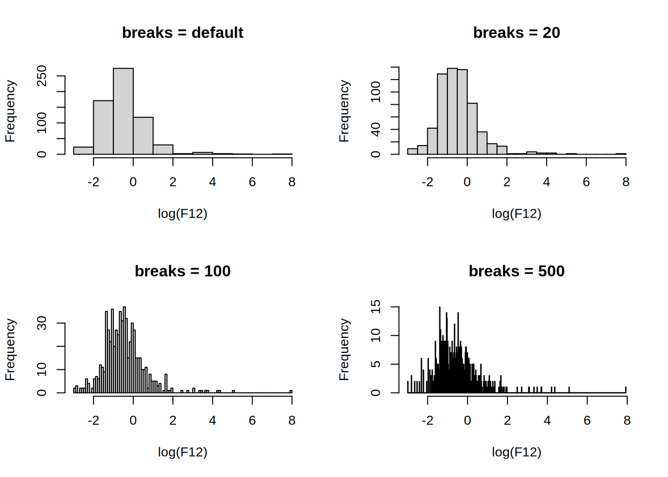
The number of breaks changes the impression of the distribution, the default uses Sturges’ formula where the number of cells for n observations is \lceil{\log_2(n)+1}\rceil.
Take away points: Read documentation to understand how the functions work, or (my preferred method) ask ChatGPT (at the cost of a higher CO2 footprint). Beware of the default arguments and implement good default values when creating functions.
Q: Write your own function, called my_breaks, which takes two arguments, x (a vector) and h (a positive integer). Let h have default value 5. The function should first sort x into increasing order and then return the vector that: starts with the smallest entry in x; contains every hth unique entry from the sorted x; ends with the largest entry in x.
A: We can try doing
my_breaks <- function(x, h = 5) {
  x <- sort(x)
  ux <- unique(x)
  i <- seq(1, length(ux), h)

  # Test if last unique element of x is included in the filter
  if (i[length(i)] < length(ux)) { # If last index not length(ux)
    i[length(i) + 1] <- length(ux) # append that index
  }
  ux[i] # index subsetting
}
x <- c(1, 3, 2, 5, 10, 11, 1, 1, 3)
h <- 2

my_breaks(x, h)
[1] 1 3 10 11Alternatively, one can write it in one-line, however this might not be the best practice, see this
my_breaks <- function(x, h = 5) (us <- unique(sort(x)))[c(seq(1, length(us), h), length(us)[!!(length(us) - 1) %% h])]Try to understand what exactly the expression length(us)[!!(length(us) - 1) %% h] does.
We can now use the function with hist()
par(mfrow = c(1, 2))
hist(log(F12), my_breaks)
hist(log(F12), function(x) my_breaks(x, 40)) # Currying (a very powerful technique)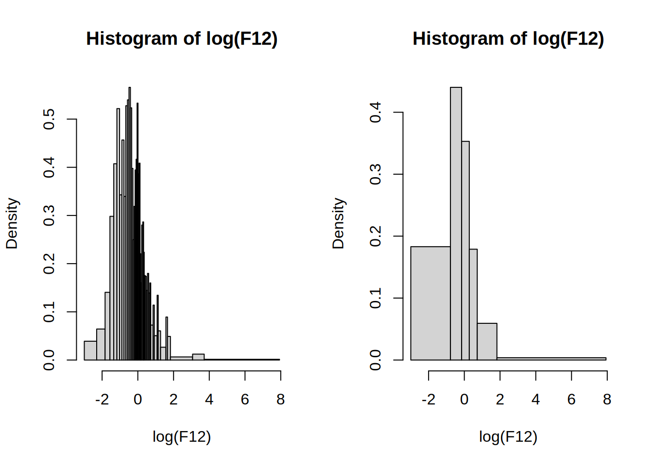
Q: If there are no ties in the dataset, the function above will produce breakpoints with h observations in the interval between two consecutive breakpoints (except the last two perhaps). If there are ties, the function will by construction return unique breakpoints, but there may be more than h observations in some intervals.
The intention is now to rewrite my_breaks so that if possible each interval contains h observations.
Modify the my_breaks function with this intention and so that is has the following properties:
x.h observations in the interval (a,b], provided h < length(x). (With the exception that for the first two breakpoints, the interval is [a,b].)A: We can do the following 2-pointer approach, where i and pointer are pointers to the current index and the next breakpoint index respectively.
my_breaks_2 <- function(x, h = 5) {
  sorted <- sort(x)
  breakpoints <- sorted[1]
  pointer <- h
  for (i in seq_along(x)[-1]) {
    if (i - pointer < 0) {
      next
    }

    if (breakpoints[length(breakpoints)] < sorted[i]) {
      breakpoints <- c(breakpoints, sorted[i])
      pointer <- i + h
    } else {
      pointer <- pointer + 1
    }
  }

  if (pointer > length(sorted)) {
    breakpoints[length(breakpoints)] <- sorted[length(sorted)]
  }
  breakpoints
}NB: Using seq_along allocates a vector from 1 to the length of the vector, which can be detrimental to performance since the CPU has to allocate memory for the vector. A better approach is to use a while loop and increment the index by 1.
Test the solution
my_breaks_2(1:2, 1) # should return 1 2[1] 1 2my_breaks_2(1:10, 5) # should return 1 5 10[1] 1 5 10my_breaks_2(1:12, 5) # should return 1 5 12[1] 1 5 12my_breaks_2(c(1, 2, 3, 4, rep(5, 10), 6), 5) # should return 1 5 6[1] 1 5 6my_breaks_2(c(1, 2, 3, 4, rep(10, 10), 11), 2) # should return 1 2 4 10 11[1] 1 2 4 10 11hh <- 1:100
breaks <- lapply(hh, function(h) my_breaks(log(F12), h))
# The number of obs in each cell
counts <- lapply(breaks, function(b) hist(log(F12), b, plot = FALSE)$counts)
# Test 1: Any cells with less than h obs?
all(sapply(hh, function(i) all(counts[[i]] < hh[i])))[1] FALSE# Test 2: Any duplicate breaks?
any(sapply(breaks, function(x) any(duplicated(x))))[1] FALSEpar(mfrow = c(2, 2))
hist(log(F12), main = "Sturges’ formula")
hist(log(F12), my_breaks_2, main = "my_breaks_2 (h = default)")
hist(log(F12), function(x) my_breaks_2(x, 10), main = "my_breaks_2 (h = 10)")
hist(log(F12), function(x) my_breaks_2(x, 50), main = "my_breaks_2 (h = 50)")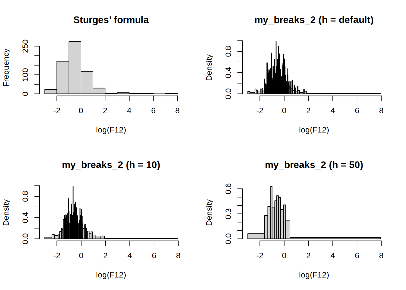
Q: Write a function called my_hist, which takes a single argument h and plots a histogram of log(F12). Extend the implementation so that any additional argument specified when calling my_hist is passed on to hist. Investigate and explain what happens when executing the following function calls.
my_hist()
my_hist(h = 5, freq = TRUE)
my_hist(h = 0)A:
my_hist <- function(h = 0, ...) hist(log(F12), breaks = function(x) my_breaks_2(x, h), ...)

my_hist()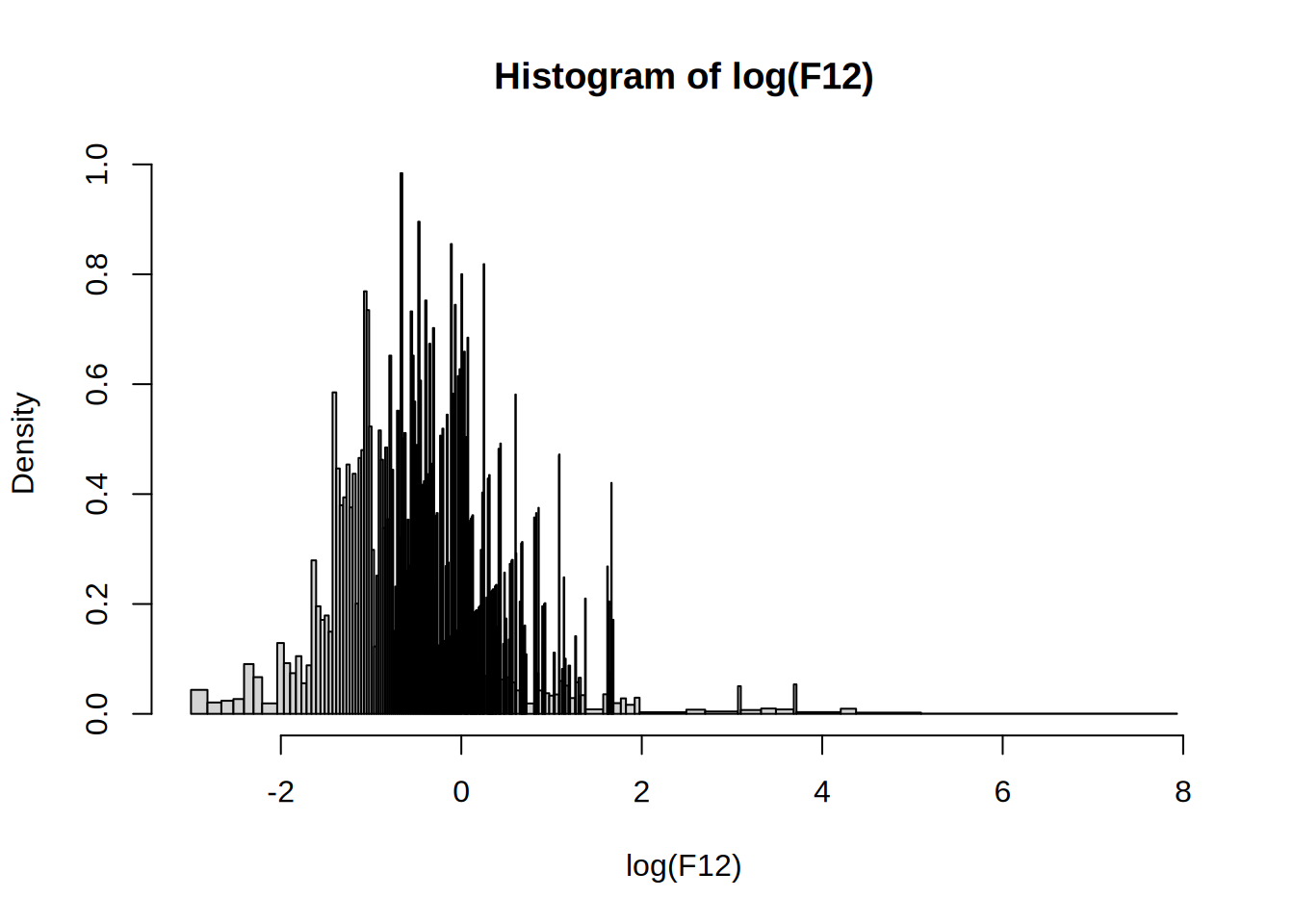
my_hist(h = 5, freq = TRUE) # fails because breaks are not equidistantWarning in plot.histogram(r, freq = freq1, col = col, border = border, angle =
angle, : the AREAS in the plot are wrong -- rather use 'freq = FALSE'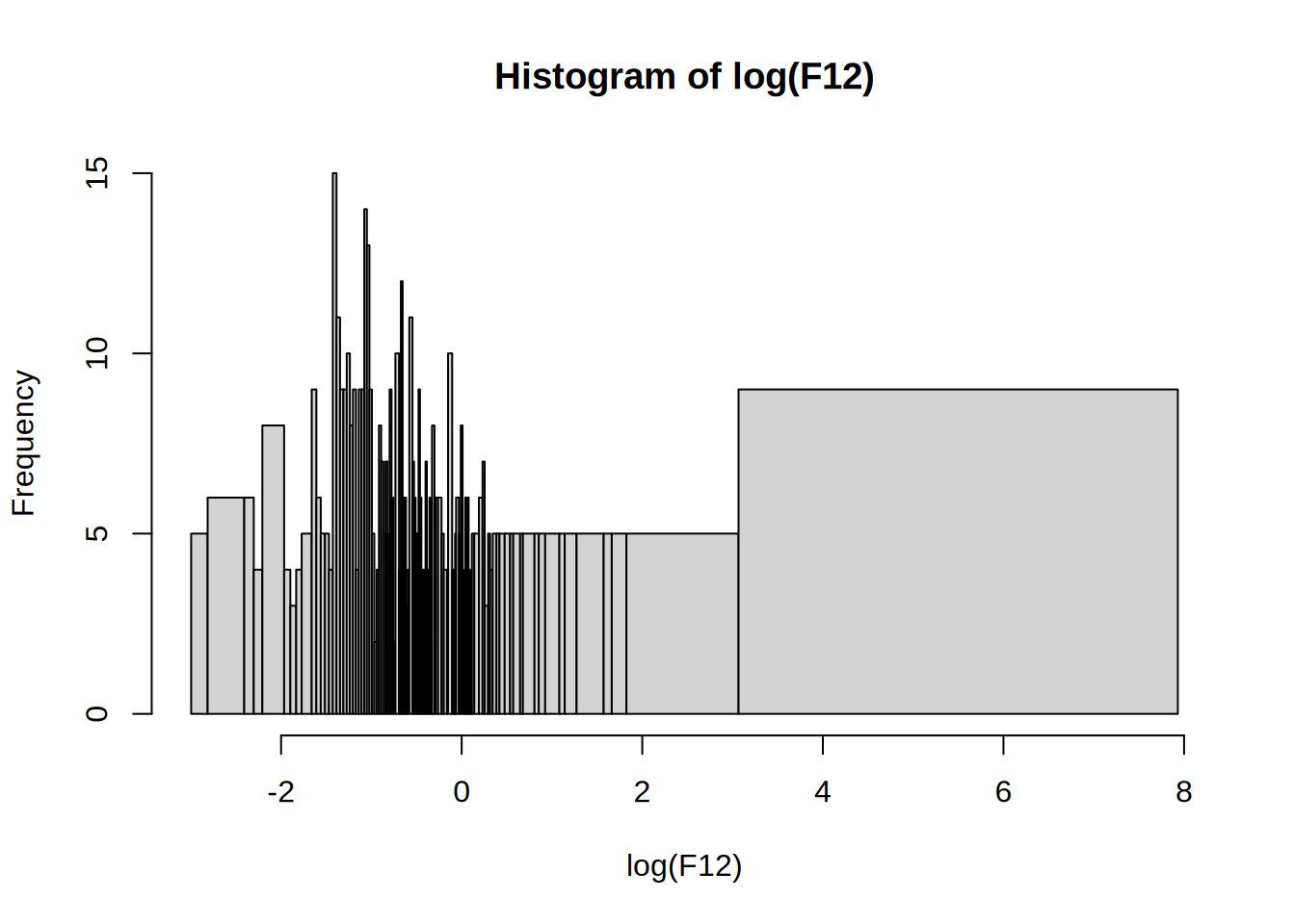
my_hist(h = 0)
Q: Modify your my_hist function so that it returns an object of class my_histogram, which is not plotted. Write a print method for objects of this class, which prints just the number of cells.
A: use structure and unclass remember plot = F
my_hist2 <- function(h = 0, ...) structure(unclass(hist(log(F12), function(x) my_breaks_2(x, h), plot = F, ...)), class = "my_histogram")Works like a charm
print.my_histogram <- function(x, ...) {
  print(paste("Number of cells:", length(x$mids)))
  invisible(x) # Q: what does invisible do?
}
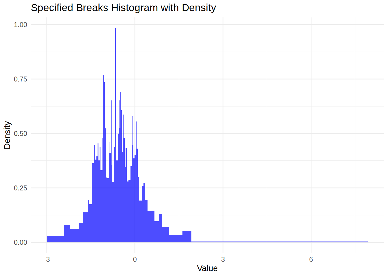
x <- my_hist2(10)Q: Write a new plot method for objects of class my_histogram that uses ggplot2 for plotting the histogram.
A: Here is one way to do it
plot.my_histogram <- function(x, ...) {
  library(ggplot2)

  breaks <- x$breaks
  density <- x$density

  data <- data.frame(
    xmin = breaks[-length(breaks)],
    xmax = breaks[-1],
    ymin = rep(0, length(density)),
    ymax = density
  )

  # Create the histogram with ggplot2 using geom_bar
  ggplot(data) +
    geom_rect(aes(xmin = xmin, xmax = xmax, ymin = ymin, ymax = ymax), fill = "blue", alpha = 0.7) +
    labs(title = "Specified Breaks Histogram with Density", x = "Value", y = "Density") +
    theme_minimal()
}

plot(my_hist2(10))